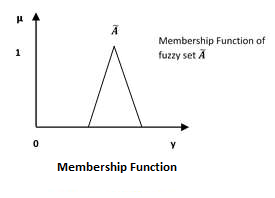
Fuzzy Logic - Membership Function and Traditional Fuzzy Refresher

Fuzzy logic is not logic that is fuzzy but logic that is used to describe fuzziness. This fuzziness is best characterized by its membership function. In other words, we can say that membership function represents the degree of truth in fuzzy logic.

Following are a few important points relating to the membership function −

• Membership functions were first introduced in 1965 by Lofti A. Zadeh in his first research paper “fuzzy sets”.

• Membership functions characterize fuzziness (i.e., all the information in fuzzy set), whether the elements in fuzzy sets are discrete or continuous.

• Membership functions can be defined as a technique to solve practical problems by experience rather than knowledge.

• Membership functions are represented by graphical forms.

• Rules for defining fuzziness are fuzzy too.

Mathematical Notation

We have already studied that a fuzzy set Ã in the universe of information U can be defined as a set of ordered pairs and it can be represented mathematically as −

A˜={(y,μA˜(y))|y∈U}$$\tilde{A}=\left\{\left(y,{\mu }_{\tilde{A}}\left(y\right)\right)|y\in U\right\}$$

Here μA˜(∙)$\mu \tilde{A}(\bullet )$ = membership function of A˜$\tilde{A}$; this assumes values in the range from 0 to 1, i.e., μA˜(∙)∈[0,1]$\mu \tilde{A}(\bullet )\in \left[0,1\right]$. The membership function μA˜(∙)$\mu \tilde{A}(\bullet )$ maps U$U$ to the membership spaceM$M$.

The dot (∙)$(\bullet )$ in the membership function described above, represents the element in a fuzzy set; whether it is discrete or continuous.

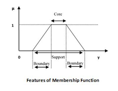
Features of Membership Functions

We will now discuss the different features of Membership Functions.

Core

For any fuzzy set A˜$\tilde{A}$, the core of a membership function is that region of universe that is characterize by full membership in the set. Hence, core consists of all those elements y$y$ of the universe of information such that,

μA˜(y)=1$${\mu }_{\tilde{A}}\left(y\right)=1$$

Support

For any fuzzy set A˜$\tilde{A}$, the support of a membership function is the region of universe that is characterize by a nonzero membership in the set. Hence core consists of all those elements y$y$ of the universe of information such that,

μA˜(y)>0$${\mu }_{\tilde{A}}\left(y\right)>0$$

Boundary

For any fuzzy set A˜$\tilde{A}$, the boundary of a membership function is the region of universe that is characterized by a nonzero but incomplete membership in the set. Hence, core consists of all those elements y$y$ of the universe of information such that,

1>μA˜(y)>0$$1>{\mu }_{\tilde{A}}\left(y\right)>0$$

Fuzzification

It may be defined as the process of transforming a crisp set to a fuzzy set or a fuzzy set to fuzzier set. Basically, this operation translates accurate crisp input values into linguistic variables.

Following are the two important methods of fuzzification −

Support Fuzzification(s-fuzzification) Method

In this method, the fuzzified set can be expressed with the help of the following relation −

A˜=μ1Q(x1)+μ2Q(x2)+...+μnQ(xn)$$\tilde{A}={\mu }_{1}Q\left(x_1\right)+{\mu }_{2}Q\left(x_2\right)+...+{\mu }_{n}Q\left(x_n\right)$$

Here the fuzzy set Q(xi)$Q\left(x_i\right)$ is called as kernel of fuzzification. This method is implemented by keeping μi${\mu }_i$ constant and xi$x_i$ being transformed to a fuzzy set Q(xi)$Q\left(x_i\right)$.

Grade Fuzzification (g-fuzzification) Method

It is quite similar to the above method but the main difference is that it kept xi$x_i$ constant and μi${\mu }_i$ is expressed as a fuzzy set.

Defuzzification

It may be defined as the process of reducing a fuzzy set into a crisp set or to convert a fuzzy member into a crisp member.

We have already studied that the fuzzification process involves conversion from crisp quantities to fuzzy quantities. In a number of engineering applications, it is necessary to defuzzify the result or rather “fuzzy result” so that it must be converted to crisp result. Mathematically, the process of Defuzzification is also called “rounding it off”.

The different methods of Defuzzification are described below −

Max-Membership Method

This method is limited to peak output functions and also known as height method. Mathematically it can be represented as follows −

μA˜(x∗)>μA˜(x)forallx∈X$${\mu }_{\tilde{A}}\left(x^{\ast }\right)>{\mu }_{\tilde{A}}\left(x\right)forallx\in X$$

Here, x∗$x^{\ast }$ is the defuzzified output.

Centroid Method

This method is also known as the center of area or the center of gravity method. Mathematically, the defuzzified output x∗$x^{\ast }$ will be represented as −

x∗=∫μA˜(x).xdx∫μA˜(x).dx$$x^{\ast }=\frac{\int {\mu }_{\tilde{A}}\left(x\right).xdx}{\int {\mu }_{\tilde{A}}\left(x\right).dx}$$

Weighted Average Method

In this method, each membership function is weighted by its maximum membership value. Mathematically, the defuzzified output x∗$x^{\ast }$ will be represented as −

x∗=∑μA˜(xi¯¯¯¯¯).xi¯¯¯¯¯∑μA˜(xi¯¯¯¯¯)$$x^{\ast }=\frac{\sum {\mu }_{\tilde{A}}\left(\overline{x_i}\right).\overline{x_i}}{\sum {\mu }_{\tilde{A}}\left(\overline{x_i}\right)}$$

Mean-Max Membership

This method is also known as the middle of the maxima. Mathematically, the defuzzified output x∗$x^{\ast }$ will be represented as −

x∗=∑i=1nxi¯¯¯¯¯n

Logic, which was originally just the study of what distinguishes sound argument from unsound argument, has now developed into a powerful and rigorous system whereby true statements can be discovered, given other statements that are already known to be true.

Predicate Logic

This logic deals with predicates, which are propositions containing variables.

A predicate is an expression of one or more variables defined on some specific domain. A predicate with variables can be made a proposition by either assigning a value to the variable or by quantifying the variable.

Following are a few examples of predicates −

• Let E(x, y) denote "x = y"
• Let X(a, b, c) denote "a + b + c = 0"
• Let M(x, y) denote "x is married to y"

Propositional Logic

A proposition is a collection of declarative statements that have either a truth value "true” or a truth value "false". A propositional consists of propositional variables and connectives. The propositional variables are dented by capital letters (A, B, etc). The connectives connect the propositional variables.

A few examples of Propositions are given below −

• "Man is Mortal", it returns truth value “TRUE”
• "12 + 9 = 3 – 2", it returns truth value “FALSE”

The following is not a Proposition −

• "A is less than 2" − It is because unless we give a specific value of A, we cannot say whether the statement is true or false.

Connectives

In propositional logic, we use the following five connectives −

• OR (∨∨)
• AND (∧∧)
• Negation/ NOT (¬¬)
• Implication / if-then (→→)
• If and only if (⇔⇔)

OR (∨∨)

The OR operation of two propositions A and B (written as A∨BA∨B) is true if at least any of the propositional variable A or B is true.

The truth table is as follows −

A	B	A ∨ B
True	True	True
True	False	True
False	True	True
False	False	False

AND (∧∧)

The AND operation of two propositions A and B (written as A∧BA∧B) is true if both the propositional variable A and B is true.

The truth table is as follows −

A	B	A ∧ B
True	True	True
True	False	False
False	True	False
False	False	False

Negation (¬¬)

The negation of a proposition A (written as ¬A¬A) is false when A is true and is true when A is false.

The truth table is as follows −

A	¬A
True	False
False	True

Implication / if-then (→→)

An implication A→BA→B is the proposition “if A, then B”. It is false if A is true and B is false. The rest cases are true.

The truth table is as follows −

A	B	A→B
True	True	True
True	False	False
False	True	True
False	False	True

If and only if (⇔⇔)

A⇔BA⇔B is a bi-conditional logical connective which is true when p and q are same, i.e., both are false or both are true.

The truth table is as follows −

A	B	A⇔B
True	True	True
True	False	False
False	True	False
False	False	True

Well Formed Formula

Well Formed Formula (wff) is a predicate holding one of the following −

• All propositional constants and propositional variables are wffs.
• If x is a variable and Y is a wff, ∀xY and ∃xY are also wff.
• Truth value and false values are wffs.
• Each atomic formula is a wff.
• All connectives connecting wffs are wffs.

Quantifiers

The variable of predicates is quantified by quantifiers. There are two types of quantifier in predicate logic −

• Universal Quantifier
• Existential Quantifier

Universal Quantifier

Universal quantifier states that the statements within its scope are true for every value of the specific variable. It is denoted by the symbol ∀.

∀xP(x) is read as for every value of x, P(x) is true.

Example − "Man is mortal" can be transformed into the propositional form ∀xP(x). Here, P(x) is the predicate which denotes that x is mortal and the universe of discourse is all men.

Existential Quantifier

Existential quantifier states that the statements within its scope are true for some values of the specific variable. It is denoted by the symbol ∃.

∃xP(x) for some values of x is read as, P(x) is true.

Example − "Some people are dishonest" can be transformed into the propositional form ∃x P(x) where P(x) is the predicate which denotes x is dishonest and the universe of discourse is some people.

Nested Quantifiers

If we use a quantifier that appears within the scope of another quantifier, it is called a nested quantifier.

Example

• ∀ a∃bP(x,y) where P(a,b) denotes a+b = 0
• ∀ a∀b∀cP(a,b,c) where P(a,b) denotes a+(b+c) = (a+b)+c

Note − ∀a∃bP(x,y) ≠ ∃a∀bP(x,y)

Anurag Rana